Explainer
Back
Our latest research on Marginal emission factors
In this blog post, we will discuss the latest advancements in our marginal technology, with the goal of assessing the immediate impact of a consumption change on the grid.

Julien Lavalley

This blog post is part of a series of articles uncovering all you need to know about marginal signals, discussing their challenges and why average emissions factors may be preferable. Find a simpler overview of the complexities to consider when using marginal signals in practice here.
The first article introduced the concept of marginal emissions factors, and the second article introduced the methodology we used at Electricity Maps to calculate marginal carbon intensity signals. In this blog post, we will discuss further developments in our marginal technology, with the goal of assessing the immediate impact of a consumption change on the grid. While we keep this article online to show the complexities of developing reliable marginal signals, we no longer offer marginal signals due to their major limitations.
Innovating on marginal - Summary

Challenges faced by existing methodologies
The marginal carbon intensity refers to the carbon intensity of the marginal power plant. Here we consider the marginal power plant the one that would provide the additional electricity requested by a consumer who decided to use slightly more electricity at a given time and location. Therefore, the marginal carbon intensity results from comparing two scenarios: one in which additional consumption happens, and one in which it doesn’t. Because one of these scenarios never happens in reality, the identity of this marginal power plant is fundamentally unobservable (read more here).
It poses a challenge: how do we determine which plant is the "marginal one"?
Is it always one physical entity, or is it a mix of power plants (several plants may increase or decrease their production simultaneously, one plant may cover the increase in the short-term and another in the mid to long-term)? Since the marginal power plant only exists when compared with a theoretical scenario, how can we ever measure if that choice is right? And how can we find the most accurate marginal model?
Because of the grid's complexity, a marginal grid mix is closer to reality than the concept of a marginal power plant and this is why most marginal models calculate a mix rather than identifying a single power plant.
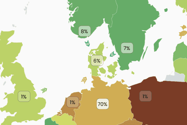
Another challenge is the impact of imports and exports on grid emissions. Significant errors are introduced when we focus on a production mix. With today’s highly interconnected grids, this is also true for marginal emissions. Additional demand could be supplied by a power plant in the same grid or somewhere else in the neighboring grids. For example, in 2023, power plants located in West Denmark contributed to only 6% of the grid’s marginal power mix while German power plants contributed to 70% of it.
Most marginal algorithms tend to disregard imports and exports and only look at electricity locally generated. However, Electricity Maps accounts for electricity exchanges with a special version of our flow-tracing algorithm.
Flow-tracing marginal flows on the grid
When we first developed our machine learning models to estimate marginal emissions at Electricity Maps, we opted for models that estimated the marginal grid mix first and derived the marginal emissions from this result.
This makes our marginal emissions models more explainable and accurate. Indeed with the importance of electricity flows in today's incredibly interconnected electricity system, this two-step approach helps us ensure electricity flows between zones are well captured. To estimate the marginal grid mix, we reused years of experience gathered from working with flow tracing algorithms to calculate consumption grid mixes worldwide.
As we strive to open our methodologies, we already discussed in greater detail how we estimate marginal carbon intensity with the combination of these two algorithms.
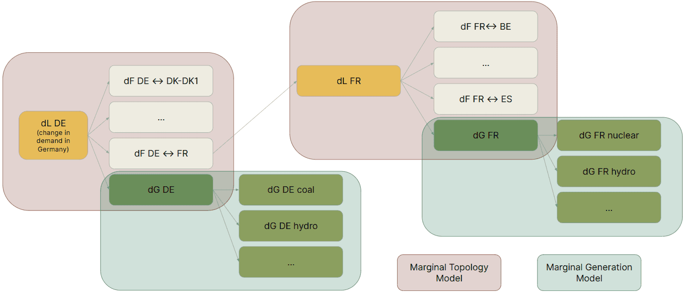
The first one called a marginal topology model, estimates how a change in load in a zone is served between a change in generation in that same zone, or a change in imports with neighboring zones. The second one called a marginal generation model, estimates how a change in generation in a zone is served between all production modes available in this zone (coal, gas, hydro, biomass, etc).
A change in exchanges with a neighboring zone affects that neighboring zone in a similar way than a load change. The marginal topology model of the neighboring zone can then be used to estimate how this change is served. Flows can therefore be traced back across the entire grid.
The combination of two machine learning models with a flow tracing methodology allows us to calculate both the marginal mix and associated marginal emissions with more accuracy by taking into account electricity flows between grids.
How do we gain confidence in marginal models
Our marginal models use machine learning to learn from historical data. The accuracy of the models represents how good they are at reconstructing past situations. However, this doesn’t mean the models will be right at understanding the consequences of an action taken on the grid. This is because machine learning models struggle to detect causality.
For example, if we were to give a list of US ice cream sales and shark attacks to a machine learning algorithm, our model could conclude that ice cream sales cause shark attacks as the two are highly correlated:

When evaluating this model it would be very good at reconstructing the past but still will be quite wrong at predicting the consequence of selling an ice cream. In this case, the validity of the model can easily be verified by an experiment. I can buy an ice cream while staying on the beach, observe that I don’t get attacked by a shark in these conditions, and conclude that the model is unfortunately wrong. However, we don’t have the luxury of experimenting with an electricity grid so we must resort to other ways.
Luckily, we can leverage the law of conservation of energy. At any point in time, the volume of electricity generated and the volume of electricity consumed on the grid must be equal. It means that when someone consumes an additional kilowatt of electricity, an additional kilowatt of electricity has to be generated somewhere on the grid (which can be far from the consumption location).
Because our models first trace back the origin of marginal electricity across the grid we can use this rule to enhance their validation. We manually recompute how electricity conservation is accounted for by our models to ensure they are not hallucinating and increase their accuracy.
Flow-tracing is critical for accurate marginal models
We’ve taken the example of West Denmark where 94% of marginal electricity comes from neighboring grids to highlight how crucial flow-tracing is for accurate marginal models. Reusing this example we emphasize how flow tracing also helps improve model validation.
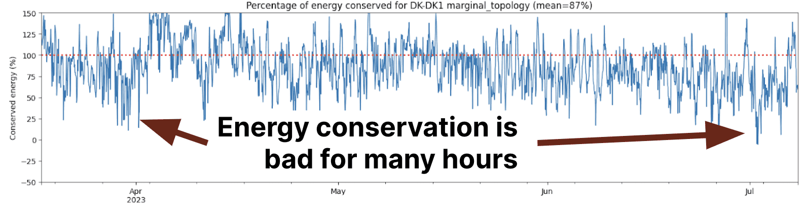
In this example, we see that the conservation of energy of our initial topology model deviates substantially from 100% which indicates that the model is not depicting a realistic situation (an additional kilowatt of demand is not served by an additional kilowatt of generation).
Looking at what caused these deviations, one can see that negative imports are detected for the Denmark-Norway interconnector. This means our algorithm is telling us that at some particular times, consuming more electricity in Denmark yields a decrease in Norwegian imports. This seems suspicious as we’d expect more electricity to be imported when increasing consumption - not less!

It represents a situation where the physics of the grid is not accurately represented anymore and hence explains why the energy conservation metric in the previous section ended up being so bad. An additional kilowatt of electricity consumed was not met by an additional kilowatt of generation in our models. But why did this happen in the first place?
Correlation ≠ Causality
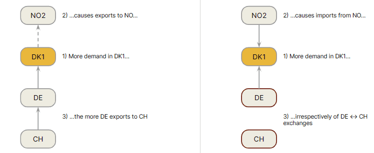
Let’s investigate here why increased electricity consumption in Denmark yields a decrease in imports from Norway (instead of an increase).
Luckily our models are explainable. Digging through the explanations, we found that these negative flows occurred every time Switzerland was exporting electricity to Germany. But what does Switzerland and Germany have to do with this?
After a long analysis which we will spare you here, we discovered that this is due to transit flows from Switzerland to Norway passing through Germany and Denmark. Historically, three increases happened at the same time:
Increased consumption in Denmark
Increased Denmark -> Norway flow
Increased Switzerland -> Germany -> Denmark -> Norway transit flow
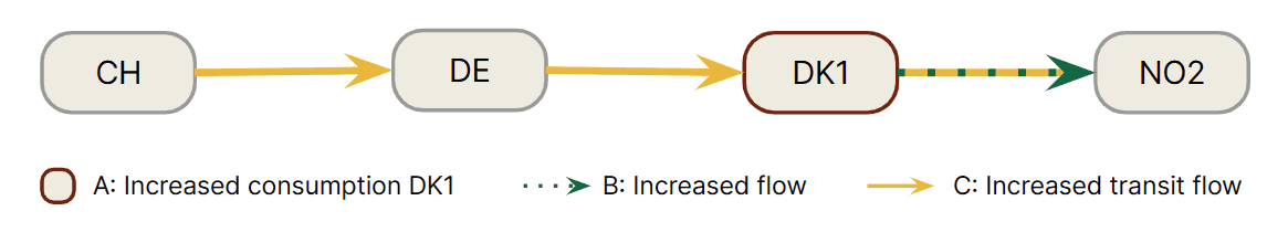
Our algorithm is mistaking correlation and causality exactly like in the example of shark attacks and ice cream sales. It tells us A is causing B because it happens at the same time whereas it is C (and not A!) that is causing B.
This discovery led us to fundamentally rethink our marginal algorithms, such that they can be better at flow-tracing causal relationships across the whole grid. This led to improving our algorithm so it is now able to detect transit flows and properly account for them. Increased consumption in Denmark now correctly leads to a positive flow (i.e. an import) from Norway and the energy conservation metric is greatly improved (a one-kilowatt increase in demand is met by a one-kilowatt increase in generation somewhere).
We already knew how important it is to account for electricity exchanges, but didn’t realize that it becomes even more important for marginal models, given their sensitivity to imports and exports. It is also important to note that these issues didn’t come up before we increased the spatial granularity of our data when we recently were able to split Norway, Denmark, Sweden, and Italy into smaller areas. This becomes crucial for the US system due to its nodal nature. Going from grid-level marginal to nodal marginal at scale is a challenge that we now are equipped to overcome.
In conclusion
Many years of marginal research have led us to understand the difficulties associated with developing a trusted and verifiable marginal signal and this methodology is the result of efforts put into better estimating marginal emissions.
We developed a new methodology adapting flow tracing to estimate the marginal grid mix before calculating marginal emissions. With this new methodology, we could propose a new validation metric: the conservation of energy. Although the identity of the marginal power plant can’t be observed empirically on the grid, this additional metric enabled us to identify situations in which our model confused correlation and causality and was thus producing wrong results. Because our models are explainable, we were able to understand the root cause and improve our models so they more accurately capture power flows on the grid.
With these changes, we are now more confident in our marginal algorithms. They incorporate the importance of exchanges. They are explainable. And, they allow us to test for their physical compatibility. These changes also allow us to flow-trace marginal signals across the whole grid at any level of resolution.
Nonetheless, marginal signals come with major limitations, such as the incompatibility with regulation, which is why we no longer offer marginal signals.
Learn more about marginal emissions factors in the others parts of this series on our blog. Read the previous part about Electricity Maps’ journey of developing models to calculate marginal carbon intensity signals, or dive into the next one about why marginal emissions are not suited for scope 2 carbon accounting.
This article had originally been published on 13/05/2024 and has been updated on 14/01/2025.

